A Second Course In Statistics Regression Analysis 7th Edition "Solution" Pdf Download UPDATED

Merrill Wherieving – March 01, 2022

• Facebook
• Twitter
• WhatsApp

A Second Course In Statistics Regression Analysis 7th Edition "Solution" Pdf Download

Linear Regression Analysis using SPSS Statistics

Introduction

Linear regression is the side by side step up after correlation. It is used when nosotros desire to predict the value of a variable based on the value of some other variable. The variable nosotros want to predict is called the dependent variable (or sometimes, the outcome variable). The variable nosotros are using to predict the other variable's value is called the independent variable (or sometimes, the predictor variable). For case, y'all could utilize linear regression to understand whether exam functioning can exist predicted based on revision time; whether cigarette consumption tin can exist predicted based on smoking elapsing; and then forth. If you have 2 or more independent variables, rather than simply ane, you need to use multiple regression.

This "quick offset" guide shows you how to carry out linear regression using SPSS Statistics, every bit well as interpret and study the results from this test. Notwithstanding, earlier we introduce you to this procedure, you need to understand the different assumptions that your data must come across in guild for linear regression to give you lot a valid issue. Nosotros hash out these assumptions next.

SPSS Statistics

Assumptions

When you choose to analyse your data using linear regression, office of the process involves checking to brand sure that the data you desire to analyse can actually be analysed using linear regression. You need to do this because it is merely appropriate to utilize linear regression if your data "passes" half-dozen assumptions that are required for linear regression to give you a valid consequence. In practice, checking for these six assumptions simply adds a fiddling flake more time to your assay, requiring y'all to click a few more buttons in SPSS Statistics when performing your assay, as well every bit remember a little bit more virtually your information, merely it is not a difficult job.

Before we introduce yous to these six assumptions, do non be surprised if, when analysing your own information using SPSS Statistics, 1 or more than of these assumptions is violated (i.e., not met). This is not uncommon when working with real-globe information rather than textbook examples, which oftentimes simply show yous how to deport out linear regression when everything goes well! Nevertheless, don't worry. Even when your data fails certain assumptions, there is often a solution to overcome this. First, let'due south accept a wait at these six assumptions:

• Assumption #1: Your 2 variables should be measured at the continuous level (i.east., they are either interval or ratio variables). Examples of continuous variables include revision time (measured in hours), intelligence (measured using IQ score), test performance (measured from 0 to 100), weight (measured in kg), and so forth. You tin can learn more near interval and ratio variables in our commodity: Types of Variable.
• Supposition #2: There needs to be a linear relationship between the two variables. Whilst there are a number of ways to check whether a linear relationship exists betwixt your 2 variables, we propose creating a scatterplot using SPSS Statistics where you can plot the dependent variable against your contained variable and then visually inspect the scatterplot to check for linearity. Your scatterplot may await something like one of the following:

  

  
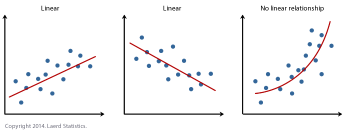
  If the relationship displayed in your scatterplot is not linear, you will have to either run a non-linear regression analysis, perform a polynomial regression or "transform" your data, which you lot tin do using SPSS Statistics. In our enhanced guides, we show you how to: (a) create a scatterplot to check for linearity when carrying out linear regression using SPSS Statistics; (b) interpret different scatterplot results; and (c) transform your data using SPSS Statistics if there is non a linear relationship between your two variables.
• Assumption #3: There should be no significant outliers. An outlier is an observed information betoken that has a dependent variable value that is very dissimilar to the value predicted by the regression equation. Equally such, an outlier volition be a point on a scatterplot that is (vertically) far abroad from the regression line indicating that it has a big residual, as highlighted below:

  

  
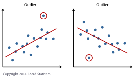
  The problem with outliers is that they can accept a negative issue on the regression analysis (eastward.chiliad., reduce the fit of the regression equation) that is used to predict the value of the dependent (effect) variable based on the independent (predictor) variable. This will alter the output that SPSS Statistics produces and reduce the predictive accuracy of your results. Fortunately, when using SPSS Statistics to run a linear regression on your data, you can easily include criteria to help you lot find possible outliers. In our enhanced linear regression guide, nosotros: (a) show y'all how to detect outliers using "casewise diagnostics", which is a simple procedure when using SPSS Statistics; and (b) discuss some of the options you have in order to deal with outliers.
• Assumption #4: You should have independence of observations, which you tin can hands cheque using the Durbin-Watson statistic, which is a unproblematic test to run using SPSS Statistics. We explain how to interpret the result of the Durbin-Watson statistic in our enhanced linear regression guide.
• Assumption #5: Your information needs to show homoscedasticity, which is where the variances forth the line of best fit remain similar as you lot move along the line. Whilst we explain more than about what this means and how to appraise the homoscedasticity of your data in our enhanced linear regression guide, take a wait at the three scatterplots beneath, which provide three simple examples: ii of data that fail the assumption (called heteroscedasticity) and 1 of information that meets this assumption (called homoscedasticity):

  

  
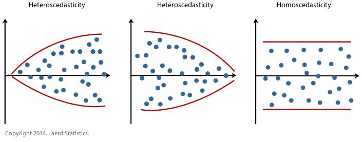
  Whilst these help to illustrate the differences in information that meets or violates the assumption of homoscedasticity, real-world data can be a lot more messy and illustrate dissimilar patterns of heteroscedasticity. Therefore, in our enhanced linear regression guide, we explain: (a) some of the things yous volition need to consider when interpreting your data; and (b) possible ways to continue with your assay if your data fails to meet this assumption.
• Assumption #6: Finally, yous need to check that the residuals (errors) of the regression line are approximately normally distributed (nosotros explicate these terms in our enhanced linear regression guide). Two mutual methods to cheque this assumption include using either a histogram (with a superimposed normal curve) or a Normal P-P Plot. Once again, in our enhanced linear regression guide, we: (a) show you how to bank check this assumption using SPSS Statistics, whether you use a histogram (with superimposed normal curve) or Normal P-P Plot; (b) explain how to interpret these diagrams; and (c) provide a possible solution if your data fails to meet this supposition.

You can cheque assumptions #ii, #iii, #iv, #5 and #6 using SPSS Statistics. Assumptions #2 should be checked first, before moving onto assumptions #three, #iv, #5 and #half dozen. We suggest testing the assumptions in this gild because assumptions #3, #4, #v and #6 require you to run the linear regression process in SPSS Statistics starting time, then information technology is easier to deal with these afterwards checking assumption #ii. Just remember that if you practice not run the statistical tests on these assumptions correctly, the results you become when running a linear regression might not be valid. This is why we dedicate a number of sections of our enhanced linear regression guide to help you lot get this right. You can find out more virtually our enhanced content as a whole on our Features: Overview folio, or more specifically, learn how we assistance with testing assumptions on our Features: Assumptions page.

In the department, Procedure, we illustrate the SPSS Statistics procedure to perform a linear regression bold that no assumptions accept been violated. Beginning, we introduce the example that is used in this guide.

SPSS Statistics

Case

A salesperson for a big machine brand wants to determine whether there is a relationship between an private's income and the price they pay for a automobile. Every bit such, the individual's "income" is the contained variable and the "price" they pay for a automobile is the dependent variable. The salesperson wants to utilize this information to determine which cars to offer potential customers in new areas where average income is known.

SPSS Statistics

Setup in SPSS Statistics

In SPSS Statistics, we created ii variables so that nosotros could enter our data: Income (the independent variable), and Price (the dependent variable). It tin can also exist useful to create a 3rd variable, caseno, to human activity equally a chronological example number. This tertiary variable is used to go far easy for you to eliminate cases (east.g., pregnant outliers) that you accept identified when checking for assumptions. However, we do not include it in the SPSS Statistics procedure that follows because we assume that you have already checked these assumptions. In our enhanced linear regression guide, we show you how to correctly enter information in SPSS Statistics to run a linear regression when you are also checking for assumptions. Y'all can acquire nigh our enhanced data setup content on our Features: Data Setup page. Alternately, see our generic, "quick start" guide: Entering Data in SPSS Statistics.

SPSS Statistics

Test Process in SPSS Statistics

The five steps below show yous how to analyse your data using linear regression in SPSS Statistics when none of the six assumptions in the previous section, Assumptions, have been violated. At the cease of these four steps, nosotros bear witness you lot how to interpret the results from your linear regression. If you are looking for aid to make certain your data meets assumptions #2, #iii, #4, #5 and #half dozen, which are required when using linear regression and can exist tested using SPSS Statistics, you tin larn more near our enhanced guides on our Features: Overview page.

Annotation: The process that follows is identical for SPSS Statistics versions 18 to 28, as well as the subscription version of SPSS Statistics, with version 28 and the subscription version being the latest versions of SPSS Statistics. Nonetheless, in version 27 and the subscription version, SPSS Statistics introduced a new expect to their interface called "SPSS Light", replacing the previous look for versions 26 and earlier versions, which was chosen "SPSS Standard". Therefore, if you accept SPSS Statistics versions 27 or 28 (or the subscription version of SPSS Statistics), the images that follow will be light grey rather than blue. All the same, the procedure is identical.

1. Click Analyze > Regression > Linear... on the elevation bill of fare, equally shown below:

   

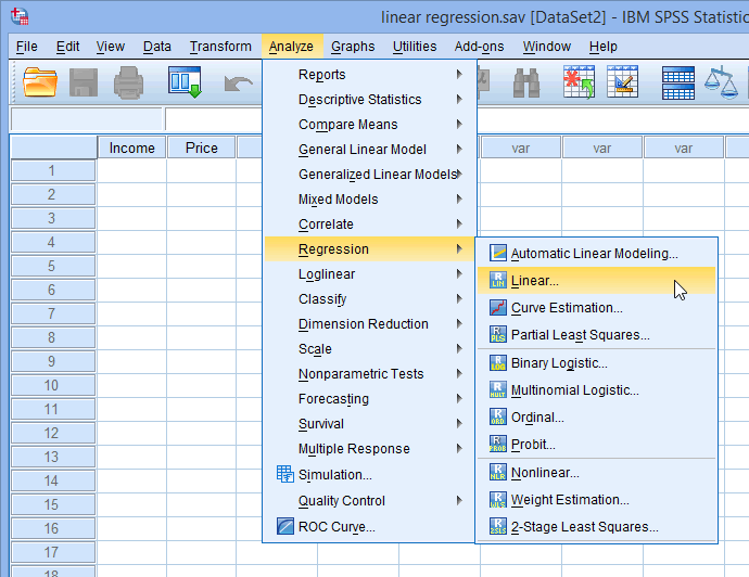
   Published with written permission from SPSS Statistics, IBM Corporation.

   You will exist presented with the Linear Regression dialogue box:

   

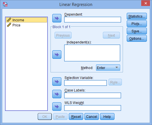
   Published with written permission from SPSS Statistics, IBM Corporation.

2. Transfer the independent variable, Income, into the Independent(s): box and the dependent variable, Price, into the Dependent: box. You can do this by either elevate-and-dropping the variables or by using the appropriate buttons. Yous will end upwardly with the following screen:

   

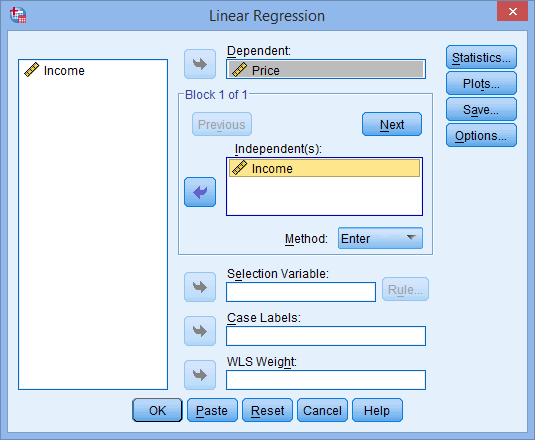
   Published with written permission from SPSS Statistics, IBM Corporation.

3. Yous now need to check 4 of the assumptions discussed in the Assumptions section to a higher place: no significant outliers (supposition #3); independence of observations (assumption #4); homoscedasticity (supposition #5); and normal distribution of errors/residuals (assumptions #6). You lot can exercise this by using the and features, then selecting the appropriate options inside these two dialogue boxes. In our enhanced linear regression guide, nosotros prove you which options to select in lodge to test whether your data meets these iv assumptions.
4. Click on the button. This will generate the results.

SPSS Statistics

Output of Linear Regression Assay

SPSS Statistics will generate quite a few tables of output for a linear regression. In this department, nosotros show you merely the three main tables required to understand your results from the linear regression procedure, assuming that no assumptions take been violated. A complete explanation of the output yous have to translate when checking your data for the six assumptions required to carry out linear regression is provided in our enhanced guide. This includes relevant scatterplots, histogram (with superimposed normal curve), Normal P-P Plot, casewise diagnostics and the Durbin-Watson statistic. Below, we focus on the results for the linear regression assay but.

The commencement table of interest is the Model Summary table, as shown below:

Published with written permission from SPSS Statistics, IBM Corporation.

This table provides the R and R ⁱⁱ values. The R value represents the elementary correlation and is 0.873 (the "R" Column), which indicates a high degree of correlation. The R ² value (the "R Square" column) indicates how much of the total variation in the dependent variable, Price, can be explained by the contained variable, Income. In this case, 76.2% can be explained, which is very large.

The next table is the ANOVA tabular array, which reports how well the regression equation fits the information (i.e., predicts the dependent variable) and is shown below:

Published with written permission from SPSS Statistics, IBM Corporation.

This table indicates that the regression model predicts the dependent variable significantly well. How practice we know this? Await at the "Regression" row and become to the "Sig." column. This indicates the statistical significance of the regression model that was run. Hither, p < 0.0005, which is less than 0.05, and indicates that, overall, the regression model statistically significantly predicts the result variable (i.e., information technology is a good fit for the data).

The Coefficients tabular array provides us with the necessary information to predict price from income, as well as make up one's mind whether income contributes statistically significantly to the model (by looking at the "Sig." cavalcade). Furthermore, we tin can employ the values in the "B" column under the "Unstandardized Coefficients" column, as shown below:

Published with written permission from SPSS Statistics, IBM Corporation.

to present the regression equation every bit:

Price = 8287 + 0.564(Income)

If you are unsure how to interpret regression equations or how to use them to make predictions, we talk over this in our enhanced linear regression guide. We besides show you lot how to write upward the results from your assumptions tests and linear regression output if you demand to written report this in a dissertation/thesis, assignment or research report. Nosotros practice this using the Harvard and APA styles. You tin can learn more nearly our enhanced content on our Features: Overview page.

We besides have a "quick start" guide on how to perform a linear regression analysis in Stata.

DOWNLOAD HERE

Posted by: killionlettemysk51.blogspot.com

• Facebook
• Twitter
• WhatsApp